A Machine-Learning Benchmark for
Semileptonic VBF Higgs-Pair Events
in a Coupling Scan

Abstract

Physics Context

Decay topology: VBF HH → bb WW* → bb qq ℓν, with two additional VBF tagging jets.

VBF Higgs-pair production is a rare process predicted by the Standard Model whose rate is highly sensitive to the quartic coupling constant κ_2V (the cvv parameter). Since VBF HH production has not yet been observed, measuring or constraining κ_2V requires ML-assisted discrimination of events produced at the SM point (cvv = 1) from events produced at anomalous coupling values.

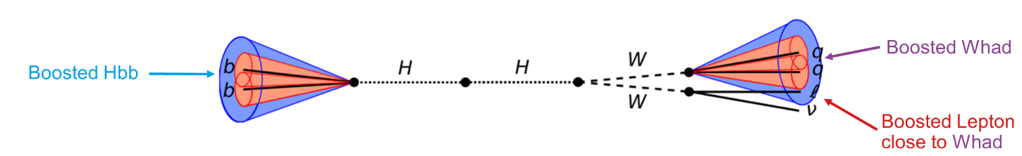
We study the semileptonic decay channel HH → bb WW* → bb qq ℓν, producing two b-jets, two light jets, a charged lepton, and a neutrino. Events are processed through a full Delphes detector simulation and jet matching pipeline. The coupling scan covers cvv ∈ {0.0, 0.5, 1.0, 1.5, 2.0, 3.0}.

Class Imbalance (after matching)

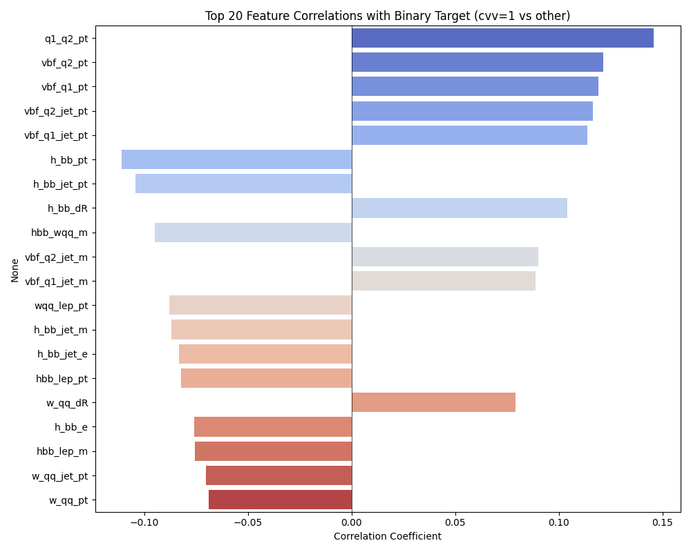
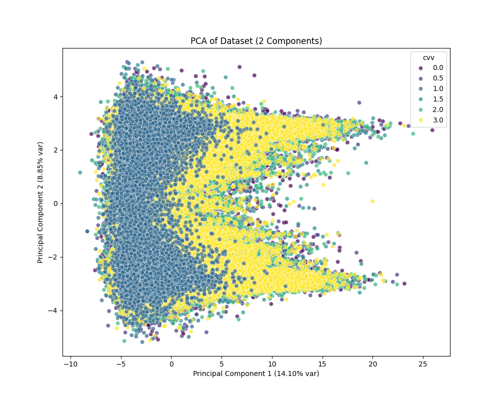
Because all non-SM classes are nearly indistinguishable from each other (5-class accuracy ≈ 20%, equal to random guessing), the task is reduced to the binary problem: C₁ vs. C_not 1.

Dataset & Features

Each event is described by kinematic four-vector observables of the reconstructed physics objects, grouped by their role in the topology. In total 52 features are used (after dropping azimuthal angles and some jet-level duplicates that provide no discriminating power). The dataset (~1M events, CSV) is publicly available for download. ↓ Download dataset

Top feature correlations with the binary target (C₁ vs C_not1). Pseudorapidity variables show the strongest discriminating power.

PCA projection of the dataset onto two principal components. The substantial class overlap reflects the fundamental difficulty of this classification task.

Feature Distributions

Select a particle and a property to explore the per-class distributions. C₁ (SM, cvv=1) is shown in red, C_not1 in blue. Most variables show substantial overlap — the coupling signal is a small shape distortion. The clearest separation appears in pseudorapidity (η) of the VBF tagging jets.

Models Overview

All classical ML models are implemented with scikit-learn and run through the same config-driven framework. The PyTorch MLP uses residual connections, batch normalisation, and optional SE blocks. DeepSets operates on sets of events.

Results

After sweeping all preprocessing combinations we identify the single best configuration per model. Toggle between the chart and a summary table below.

Chart Table

Best validation accuracy per method across all ablation configurations. Sampling strategy and scaling are annotated inside each bar.

Method	Best Accuracy	Best Sampling	Best Scaling
MLP Classifier	78.64%	3× Oversample	STD
Gradient Boosting	77.86%	Undersampled	STD
HistGradient Boosting	77.84%	Undersampled	STD
Polynomial LR	77.62%	3× Oversample	STD+L2
Random Forest	77.57%	3× Oversample	STD
DeepSet (single event)	77.58%	Single Event	STD
Nystroem-SGD	77.53%	3× Oversample	Yeo-Johnson
Voting Classifier	77.32%	Undersampled	STD
Logistic Regression	77.01%	3× Oversample	MaxAbs
SGD Classifier	76.67%	3× Oversample	STD+L2
LDA	76.46%	3× Oversample	STD+Max
Bagging Classifier	76.44%	Undersampled	STD
Gaussian NB	73.95%	3× Oversample	Quantile

Key Findings

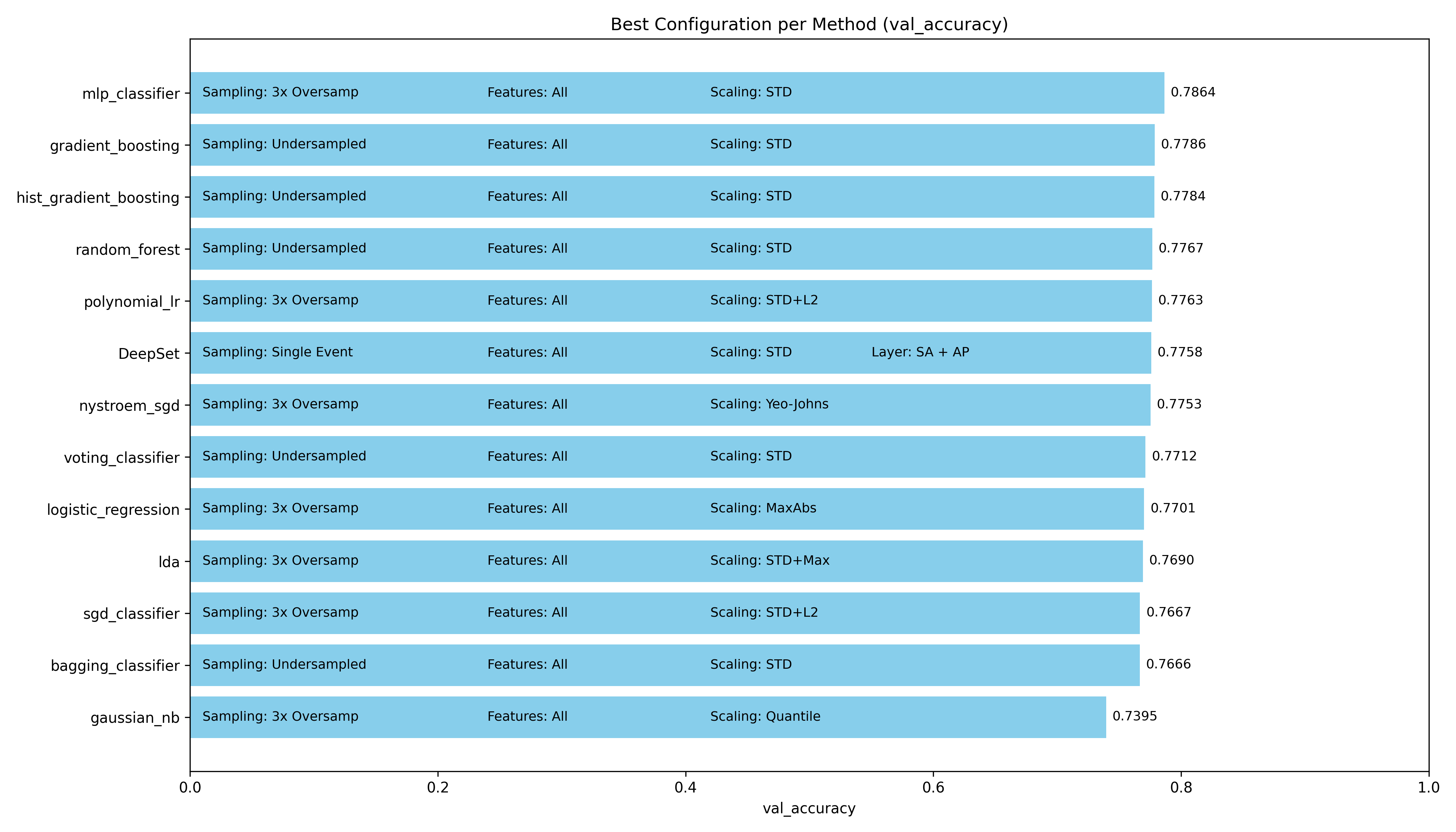
• All models cluster tightly in the 74–79% range when tuned to their best settings, suggesting the bottleneck is the data rather than the choice of model.
• The MLP achieves the highest accuracy at 78.64%, outperforming the second-best (Gradient Boosting, 77.86%) by only 0.78 percentage points.
• Standard scaling + 3× oversampling is the most common winning preprocessing combination across models.
• Gaussian NB is the clear outlier, limited by its Gaussian feature assumption, but still reaches 74%.

Feature scaling transforms each column to a common numerical range before training. We compare 7 strategies: Standard (STD), MinMax, MaxAbs, Robust, Yeo-Johnson, Quantile (normal), and Quantile (uniform). For neural networks and distance-based methods, scaling is critical because gradient updates are dominated by large-magnitude features otherwise. Tree-based models are theoretically invariant but can still be affected in practice through interaction with regularization.

Validation accuracy of all models grouped by scaling strategy. Each cluster of bars is one method; colours indicate scaling variant.

Relative accuracy difference versus the no scaling baseline. Positive values indicate improvement over no scaling.

Key Findings

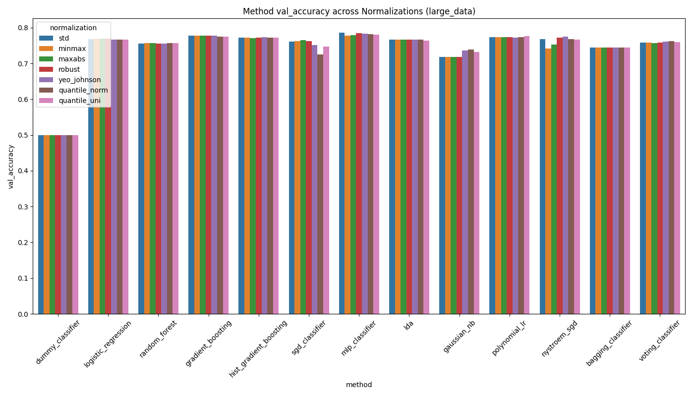
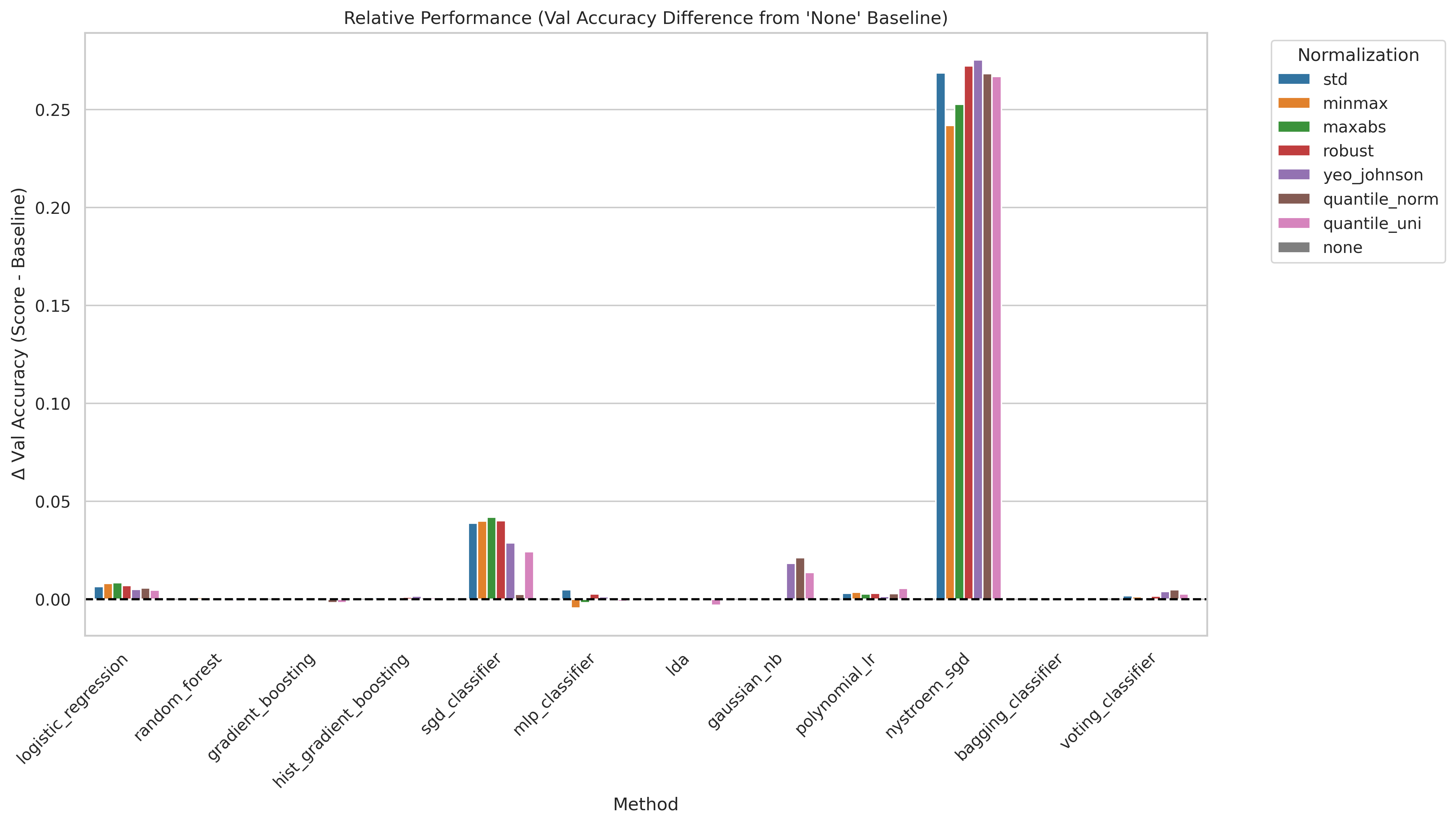
• Standard scaling is a safe default — it either wins or ties with more exotic strategies for nearly every model.
• Tree-based models (Random Forest, Gradient Boosting) are largely insensitive to the scaling choice, as expected from their split-based nature.
• The MLP benefits most from standard scaling; Yeo-Johnson and quantile transforms offer no consistent improvement and occasionally hurt.
• Gaussian NB is an exception: it benefits from quantile normalization because its Gaussian assumption is better satisfied after that transform.

Per-sample (row-wise) normalization scales each individual event vector to unit norm after column-wise scaling. We test four variants: no normalization, L1 norm, L2 norm, and Max norm. The idea is to remove scale differences between events, which can help when the overall magnitude of a feature vector carries no class-discriminating information.

Validation accuracy across normalization variants for each model.

Relative accuracy difference versus no per-sample normalization. Positive means normalization helped.

Key Findings

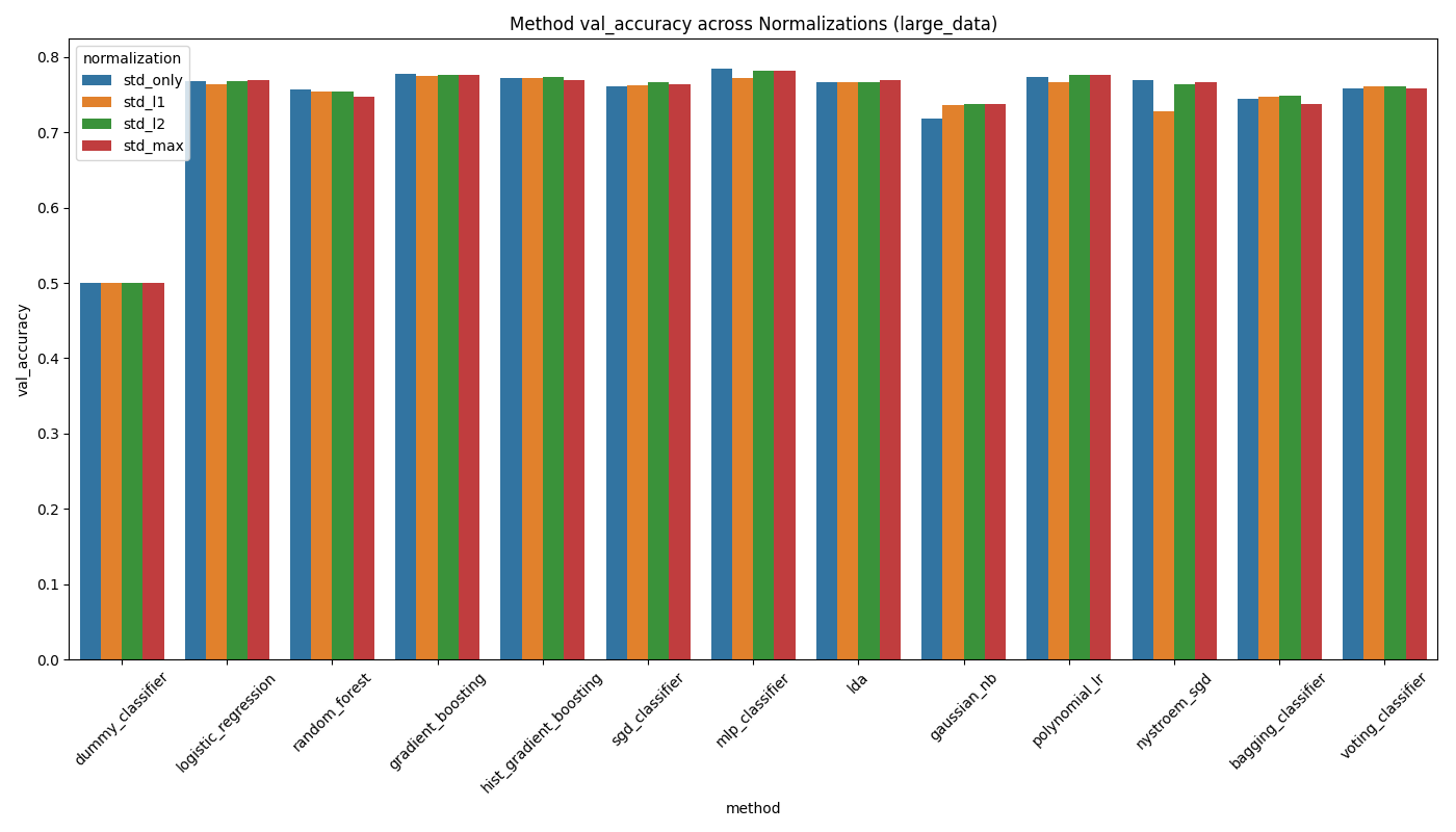
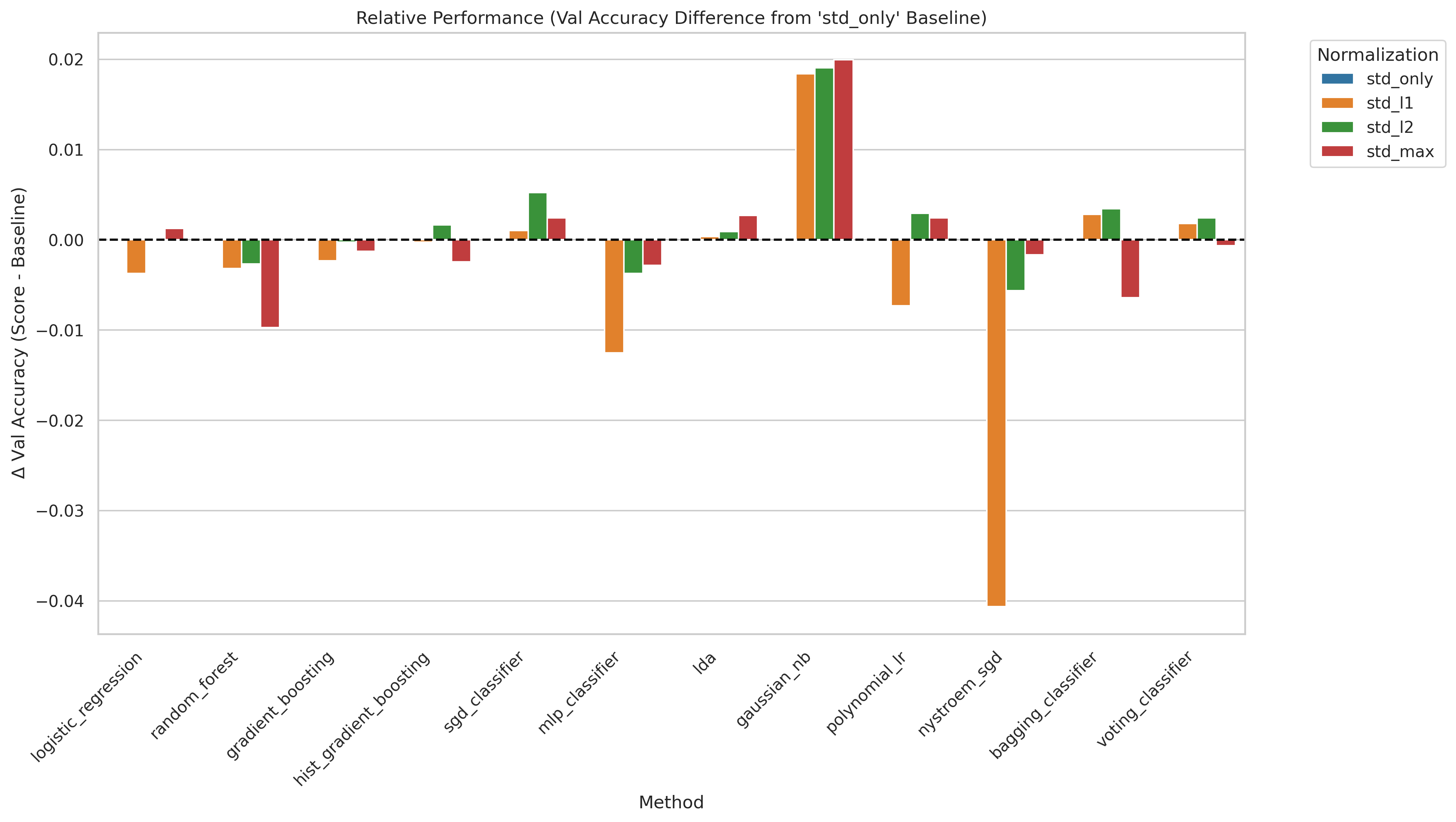
• Per-sample normalization provides no meaningful benefit for most models — the differences are within noise.
• Only Gaussian NB shows a consistent improvement with L2 normalization, because normalizing the event vector better satisfies its independence and Gaussian assumptions.
• For some models (MLP, GBT) normalization slightly hurts, likely because it destroys the absolute scale information that carries class-relevant signal (e.g., total event energy).
• Recommendation: skip per-sample normalization unless specifically using Gaussian NB.

We compare three feature sets: all features (52 variables including combination observables), old features (basic kinematic four-vectors only, no derived quantities), and new features (the combination observables alone). The combination features are derived quantities involving multiple reconstructed objects — such as the HH invariant mass, ΔR distances between systems, and multi-object invariant masses — motivated by their expected sensitivity to the coupling structure.

Validation accuracy for each model and feature set combination.

Relative accuracy change when comparing against the basic feature set.

Key Findings

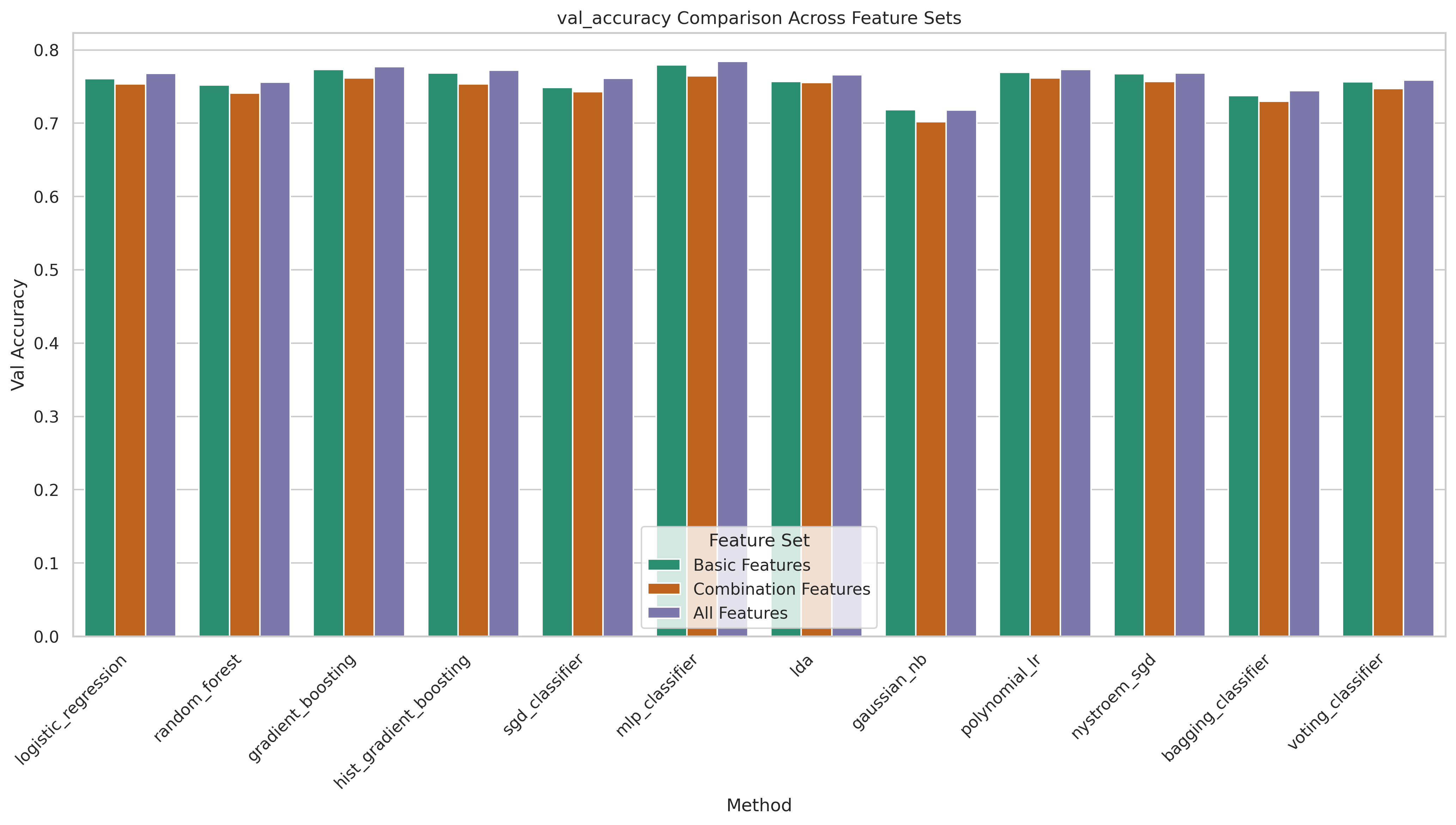
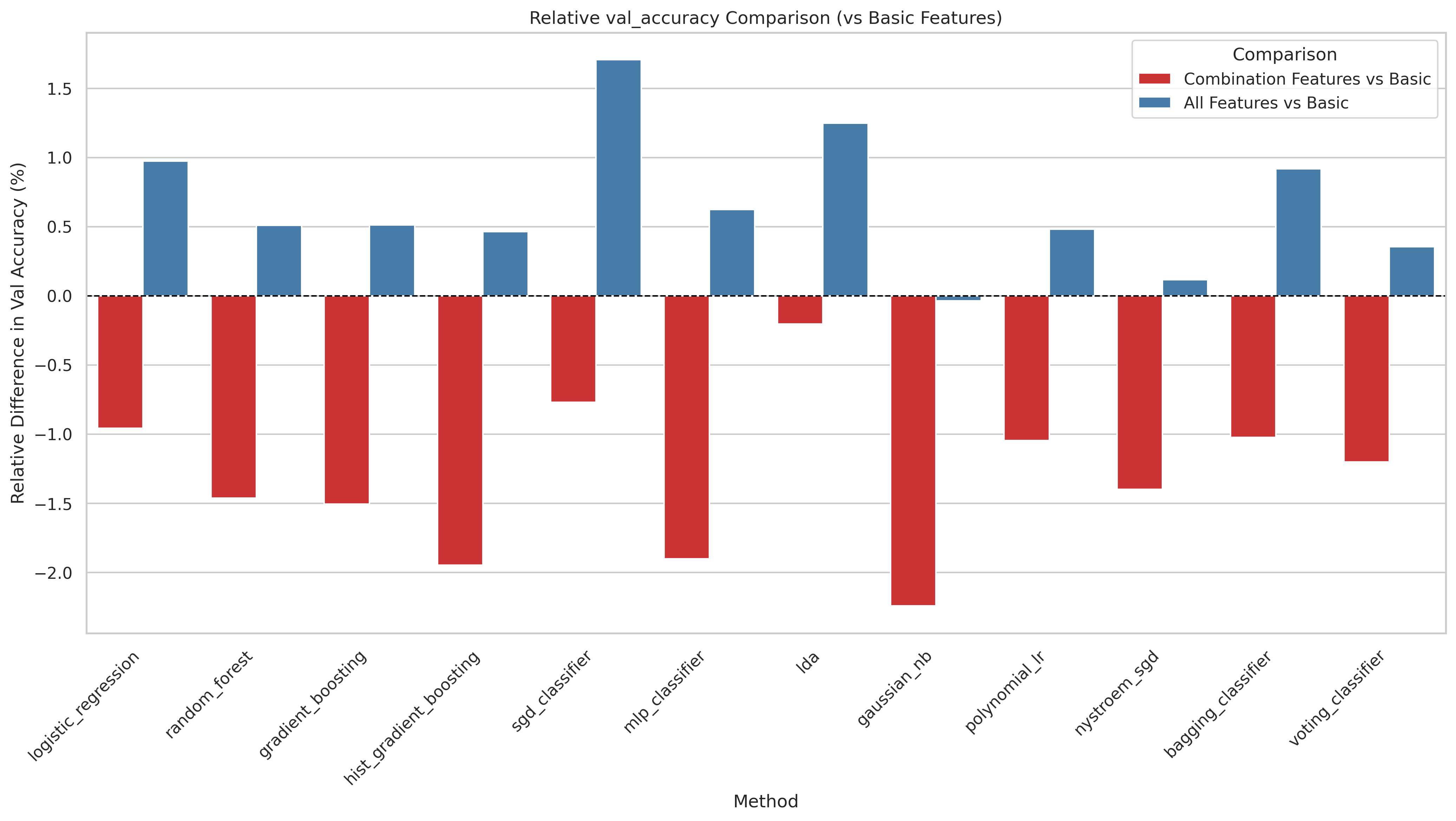
• Using all features is consistently the best or tied-best choice.
• Combination features add up to ~1.7% accuracy for some models over basic kinematics alone.
• The combination features alone (without basic kinematics) perform significantly worse, confirming they complement rather than replace the basic four-vector information.

The Standard Model class (cvv = 1) has only 0.4% matching survival, leading to a severe class imbalance. We compare three strategies: undersampling (reducing the majority class to match the minority), 3× oversampling (SMOTE-style duplication of the minority class to 3× its original size), and 10× oversampling.

Validation accuracy per model under each sampling strategy.

Relative accuracy improvement versus the undersampling baseline.

Key Findings

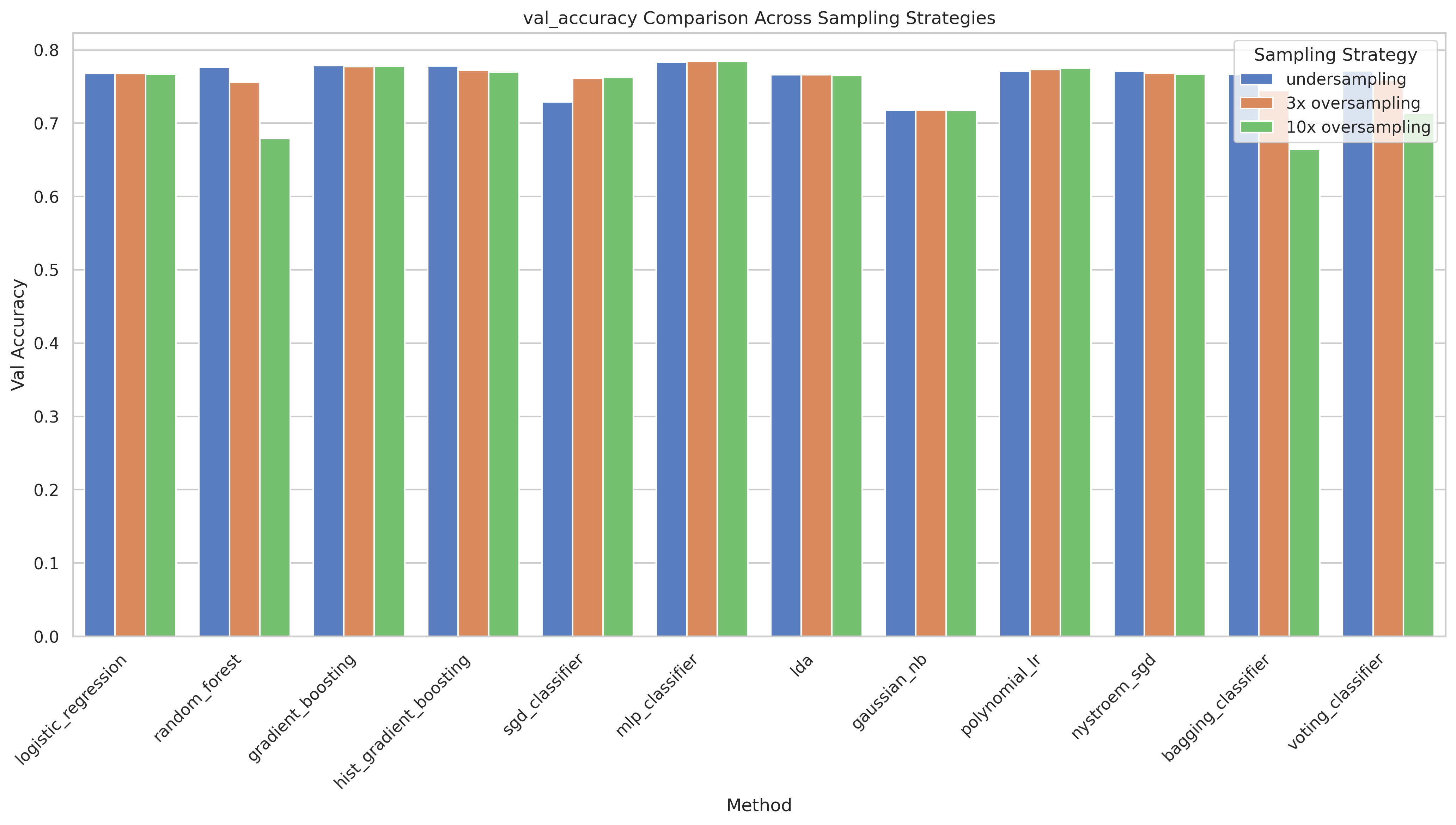
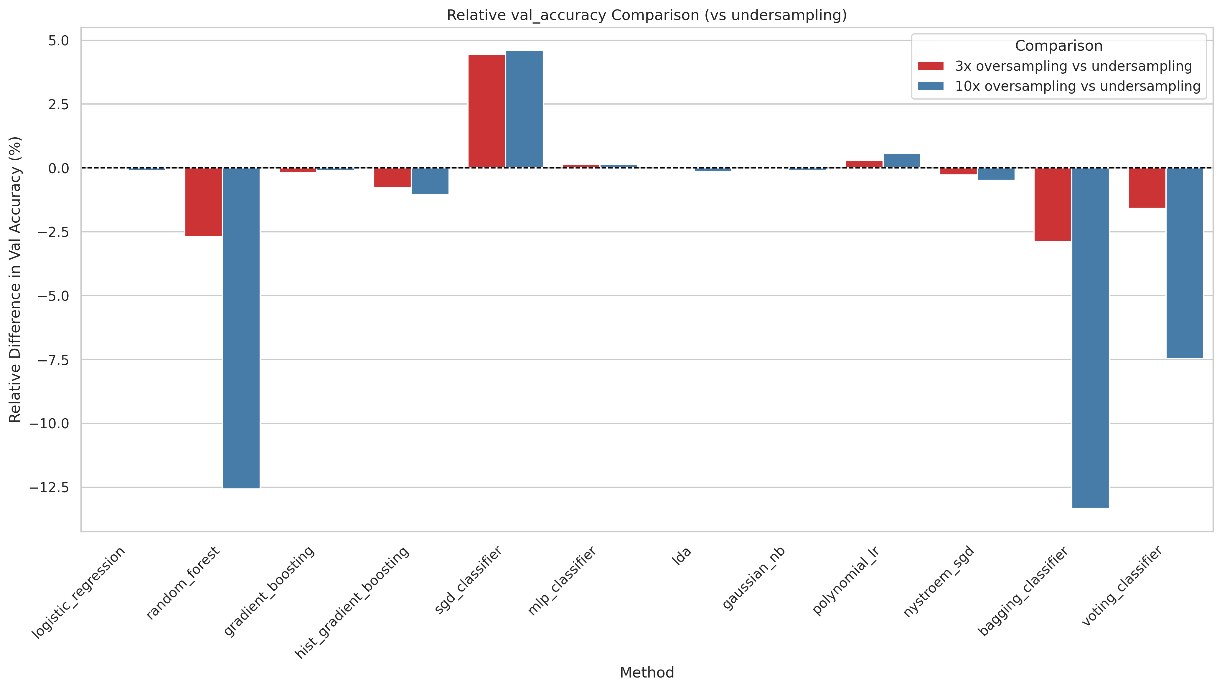
• 3× oversampling surprisingly only improves the SGD classifier significantly. This suggests that more data from the majority class doesn't improve performance.
• Undersampling is surprisingly competitive and wins for tree-based models (GB, HistGBT, Random Forest), likely because it produces a cleaner, balanced dataset that those methods handle well.
• 10× oversampling consistently hurts: the minority class is repeated so many times that models memorize it, leading to overfitting and worse generalization.

Ensemble methods combine predictions from multiple individually trained models via majority voting. The idea is that if models make different errors, a vote can cancel individual mistakes and improve overall accuracy. We test diverse combinations of the best-performing models (MLP, GBT, HistGBT, Random Forest, Logistic Regression) and measure both accuracy and macro F1 of the ensemble versus the individual member models.

Ensemble validation accuracy for different model combinations versus individual model baselines.

Ensemble macro F1 for the same combinations.

Key Findings

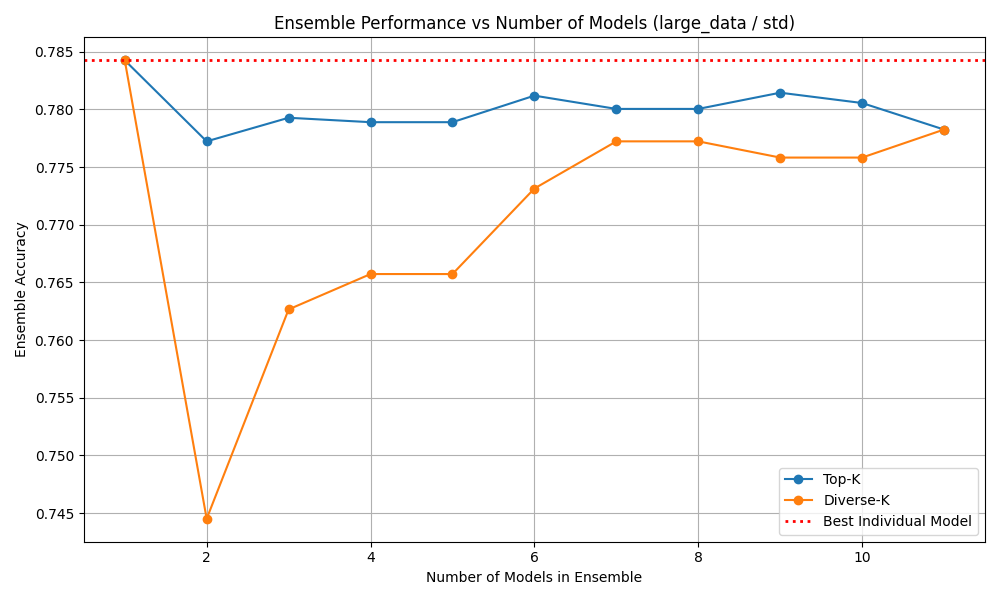
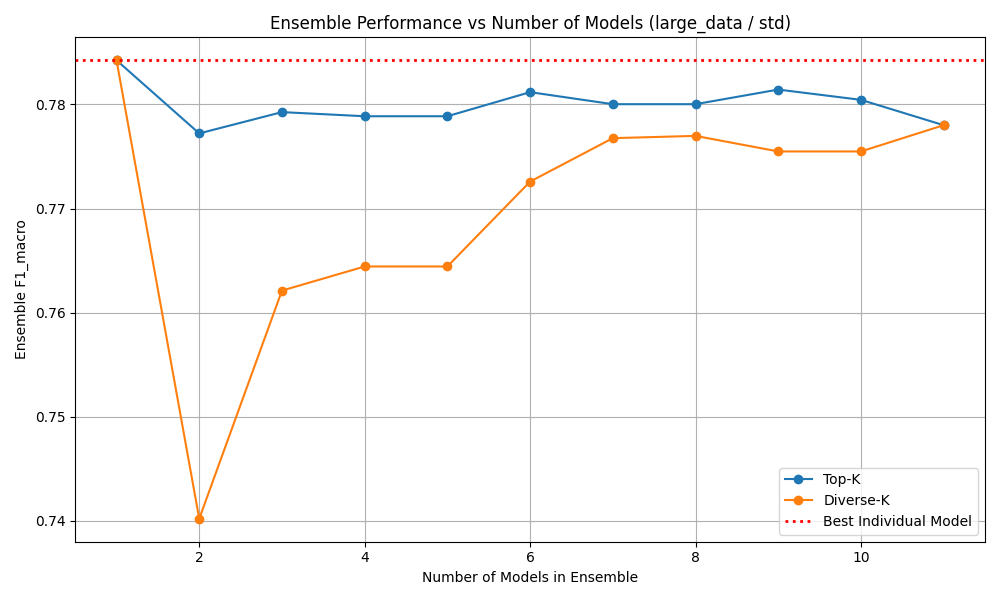
• No ensemble combination outperforms the best individual model. The MLP alone at 78.64% is not beaten by any voting ensemble.
• High pairwise model agreement (≥ 92% for MLP + GBT) leaves no room for diversification — all models agree on the same predictions, both correct and incorrect.
• This strongly implies that the models all learn from the same feature structure and hit the same information ceiling imposed by the data.
• Ensemble methods are not a viable path to improving performance on this task without fundamentally new information (e.g., multiple events).

Conclusion & Outlook

This study demonstrates that binary discrimination of VBF HH events at the Standard Model coupling point from all other coupling values is achievable with classical ML, but is genuinely difficult due to extreme class imbalance and limited signal in single-event representations.

Standard scaling and 3× minority oversampling form a robust preprocessing baseline. Adding combination features (derived multi-object quantities) gives small but consistent improvements. No ensemble combination outperforms the best individual model, confirming that all methods exploit the same feature correlations.

The most striking result is from DeepSets: classifying sets of 10 events simultaneously reaches 99.1% accuracy, compared to 77.6% for a single event. This suggests that while the coupling signal in a single event is weak, it becomes highly statistically significant when integrated over multiple events — exactly the situation in a real experimental analysis.

Limitations & Future Work

All results are based on truth-level simulation without detector effects. No held-out test set was used; all reported numbers come from the validation split. Future work could apply the framework to detector-level data, use larger datasets, or investigate whether the strong DeepSets results hold under more realistic experimental conditions.

@techreport{benchmark2025vbf,
  author    = {Foerster, Felix and Schneider, Lars and Mesner, Johannes and Linden, Lars and Stauch, Celine},
  title     = {A Machine-Learning Benchmark for Semileptonic VBF Higgs-Pair
               Events in a Coupling Scan},
  institution = {Technical University of Munich / LMU Munich},
  year      = {2025},
  url       = {https://spatenfe.github.io/vbf_event_classifier/}
}